Mouse Brain Atlas Tutorial

Mouse Brain Atlas Tutorial

1.
Download the Sample Atlas

This archive contains the images and HTML documents required to create an atlas of your own. It is based on our Mouse Brain Atlases. You will need a copy of Photoshop 3.0 or later to view our sample atlas with these tutorial files.

Library Folder
Download the sample horizontal atlas.
(53 MB: ZIP archive)

Included are a photoshop document containg a stack of images, custom HTML code for serving the files, and this help file.

Virtually all of the high-resolution images required to make atlases can be obtained from the Mouse Brain Library. High contrast images of sections are available for over 120 mice and over 62 strains in horizontal and coronal planes. For example, you could make your own atlas of an aged mouse brain or of a particular strain that interests you. If you would like to add your atlas to our collection please contact Rob Williams.

Open and Load Atlas Documents

Decompress the archive dowloaded in Step One.
We have made extensive use of Photoshop's ability to manipulate multiple layers. All of the images for one atlas are contained in the main stack until they are exported for use on the web.
Run Photoshop (version 3.0 or later) and open the file "atlas_template.psd" (this file is very large, so it may take a few minutes to load). For the sake of size, we have removed most of the layers from this atlas file. The remaining sections should provide a useful template for your atlas.

Structure of the Photoshop Stack

Each section image has its own layer. The labels for each section are contained in a separate layer. This organization scheme gives a high degree of flexibility. Sections can be easily replaced and realigned with minimal changes to the atlas as a whole.
The atlas contains two grids. The real grid gives measurements of the actual size of the tissue while the in-vivo grid compensates for shrinkage that occured during fixation. These values will vary depending on the brain and size of the images. They can be easily calculated by analyzing the size of the image and the real size of the physical brain.

Importing New Images

Now that you are familiar with the structure of the Photoshop file, it is time to import the images for your atlas. This can be done in several ways. Generally you will open the images in Photoshop and move them into the already open atlas file.
Do not worry if the new images are not the same size as the template images. The templates will eventually be removed altogether.

Alignment and Image Quality

As you import the images, you should pay attention to their quality. Certain Photoshop functions can often improve the quality of images. There is no single formula or process that obtains the highest quality from an image, it is really left to the discretion of the user.
The Adjust option under the Image menu contains many useful tools. Selecting Levels... brings up a histogram that shows a graph of the number of pixels at each brightness level. There will often be empty space at each end of the graph. If this is the case move the triangular sliders along the bottom of the graph until there are fewer unused brightness levels. Photoshop will preview the effects of your changes in the background. Adjusting the contrast is also often quite helpful.
Once all of the images are in the file, it is necessary to align them. Using Photoshop's guides, create a frame of reference to use when aligning the images. More precise adjustments can then be made by cycling through the sections in order. Holding Down the Option key and dragging will move the current layer.
If the sections need to be rotated to gain proper alignment, select the Measure Tool and draw a line down the central vertical axis of the image. Then select R otate Canvas - Arbitrary from the Images menu. The default value will come from the angle that the line makes with the perpendicular. Continue to rotate the image until you are pleased with its alignment.

Labeling

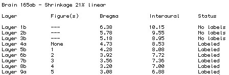
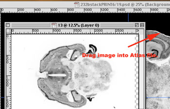
Now that the images are in the proper order and of the desired quality, it is time to begin the labeling process. In our atlases, we have adopted the naming conventions used in The Mouse Brain In Stereotaxic Coordinates by Paxinos and Watson. A list of the abbreviations is available online.
We must first create a text layer to contain the labels for the section. Select the text tool and click in the approximate area of the structure that you would like to label. In the resulting window, type the abbreviation for the structure. Using the Move Tool drag the label to the appropriate structure.
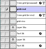
Since this is the first label, it is necessary to render the layer so that other layers may be merged on to it. In the Layer menu, select Type - Render Layer. The icon on the layer in the list of layers will change once it has been rendered.
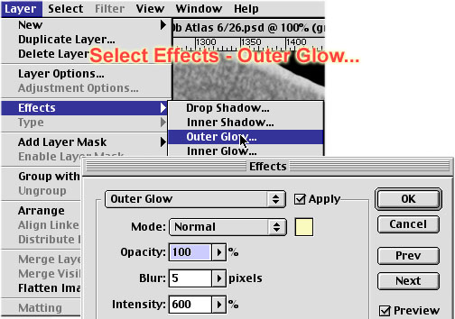
So that the labels will standout against the background of the brain, we will apply an outer glow to everything in the text layer. Make sure that the current text layer is still selected and choose Effects - Outer Glow from the Layer menu. Select Normal Mode and experiment with the other settings until you obtain the desired result.
We now have a text layer for this section. At this point, its name is still whatever abbreviation you typed earlier. Double click on the layer in the list of layers and give it a more descriptive name.
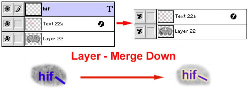
Select the Text Tool again and label the next structure. You will notice that this will create a new layer. Once you have placed this label in its proper position choose Merge Down from the Layers menu. This will combine this layer with the one below it (hopefully that is still the section's text layer). Since the new label is now part of the text layer it will take on the outer glow of all objects in that layer.
Sometimes drawing lines from a label to a structure adds clarity. If this is necessary, select the Line Tool and draw the line. It too will take on the outer glow of the text layer.
References: For the identification of structures in the mouse brain we refer the user to:
- The Mouse Brain in Stereotaxic Coordinates (1997) K. Franklin, G. Paxinos, Academic Press, San Diego. ISBN Number 0-12-26607-6. (Library of Congress: QL937.F72).
- A Stereotaxic Atlas of the Albino Mouse Forebrain (1975) B. M. Slotnick, C. M. Leonard. U.S. Department of Health, Education and Welfare, Rockville, MD.

Grids and Coordinates

You now must determine the stereotaxic coordinates for each section. It is helpful to look at other atlases when determining new coordinates. This can normalize the values in your atlas and help to eliminate any oddities specific to the subject brain. It is advisable to create a file with a list of all the sections and their coordinates. A sample file (Status) is included with the archive. This file provides an easy reference for analyzing the location and status of a slide.
Now that we have coordinates for each slide, we need to place them on the section itself. This can be accomplished using the text tool and then merging the layer down to the image layer. It is important to have this information on the image itself since it will often be viewed outside of the web page.
To be sure that the grids are acurate for your images you should create a ratio of the actual size of the brain section to the number of pixels that it takes up on the screen. You can then use this ratio to resize the grid images to the proper size. Select The in-vivo grid compensates for linear shrinkage. Use the shrinkage value obtained in Step 8 to resize the in-vivo grid.

Calculate the Linear Shrinkage

During the fixation process, the brain undergoes a substantial amount of shrinkage. To calculate shrinkage you need to know the processed brain volume and the initial brain weight prior to processing. (You can obtain original brain weights from the Mouse Brain Library.) Here is an example of computing shrinkage: a brain weighs 450 mg immediately after dissection. Since mouse brains have a density that is only slightly denser than water we can directly convert this weight to a volume of 450 mm³. After processing, we establish by point-counting or planimetry of one of the slides in the MBL that the volume of this processed brain is 150 mm³. A simple example of how to determine volume by point counting is provided in a recent review (Williams, 2000).
We now take the ratio of the processed volume over the original volume, in this case 150/450. This is a direct estimate of the remaining volume (obviously, one-third), and the volumetric shrinkage is simply 1.00 – 0.33. Take the cube root of 0.33 and subtract this value (~0.69) from 1.00 to get an estimate of linear shrinkage; 31% in this case.
In vivo grid dimensions should be 31% smaller than those of the real grid. This reduction can be done precisely by selecting the "Edit--Transform--Numeric..." command in Photoshop and entering the scaling factor.

Exporting Images for use on the Web

Once you are pleased with the appearance and accuracy of your new atlas, you can begin to export the images for the web. Before proceeding, you should become familiar with the layout of the web atlas. As you can see you will usually need to export eight different images for each section. There will be four small preview images (approx. 450x350) and four large (full-size) images.
Since there are often 30 to 40 sections in a single atlas there could be as many as 320 images to export. While this number sounds quite daunting, you can use the ability of Photoshop to batch process files to greatly reduce the amount of time this will take. For more information on actions and batch processing see your Photoshop manual.
It is a good idea to plan the structure of your HTML hierarchy before beginning to export the images. This way you will be sure to name and save them in a way that will make any unforseen changes fairly simple.

10.

Creating HTML Files

We have included a sample atlas directory with HTML and image files. This is intended to give an idea of the structure of the atlas. Please feel free to edit the files to suit your needs.
The HTML files for each section are identical except for the references to specific images. This makes it very easy to generate HTML files quickly and then search and replace to make the necessary changes.

A Human Brain Project/Neuroinformatics program funded by the National Institute of Mental Health,
National Institute on Drug Abuse, and the National Science Foundation (P20-MH 62009).
Web server statistics report since October 11, 2004 is available here
This page has been visited times! since 12-9-2005
© Copyright 2003 mbl.org