Imaging Techniques and Calibration

All brains currently in the MBL were cut at a setting of 30 µm in either the coronal or horizontal planes and were subsequently stained with cresyl violet—an analine dye that preferentially stains RNA and DNA.

Slides and sections were initially imaged with a Micro Nikkor 60 mm camera lens. Images were digitized using a Kodak DCS460 digital camera in 16-bit gray scale mode. The CCD has a pixel count of 3060 by 2036. These digital images were transferred to Adobe Photoshop. Image contrast was optimized in 16-bit mode and then reduced to 8 bits.

New Systems. We now image all slides using a Phase One LightPhase digital camera back (resolution of 3056 by 2032 pixels, 32-bit color). The camera back is mounted to a KaptureGroup TrueWide camera body that accepts almost all standard 35 mm objectives. The digital camera is connected via FireWire to a Macintosh G4. For low power work we use the same 60 mm Micro Mikkor f2.8 lens at an aperature of f8 as described above. For higher power color imaging (3.5 µm/pixel) we now use a Schneider Kreuznach Apo-Componon F2.8 40 mm Macro enlarger lens in a reverse orientation (the slide is put where the negative usually would be put). The lens is atached to a Nikon PB-6 bellows with about 100 mm of extension. This new system gives extraordinarily sharp images (see our new DBA/2J Brain Atlas).

We have now upgraded to a 4080 x 4080 LightPhase H20 digital camera back system to increase resolution to about 2.5 µm per pixel.

Several types of images have been generated. Most images are contrast-optimized 8-bit grayscale images that have been compressed and saved as high quality JPEGs (quality level 8 or 9). At their highest resolution, these compressed images take up about 0.6 to 1 megabyte. They are intended to be downloaded and viewed using Image/J, NIH Image, IPLab Spectrum (Scanalytics Inc.), or Photoshop. These JPEG images can also be viewed directly within your Web browser, but only at a 1:1 pixel ratio.

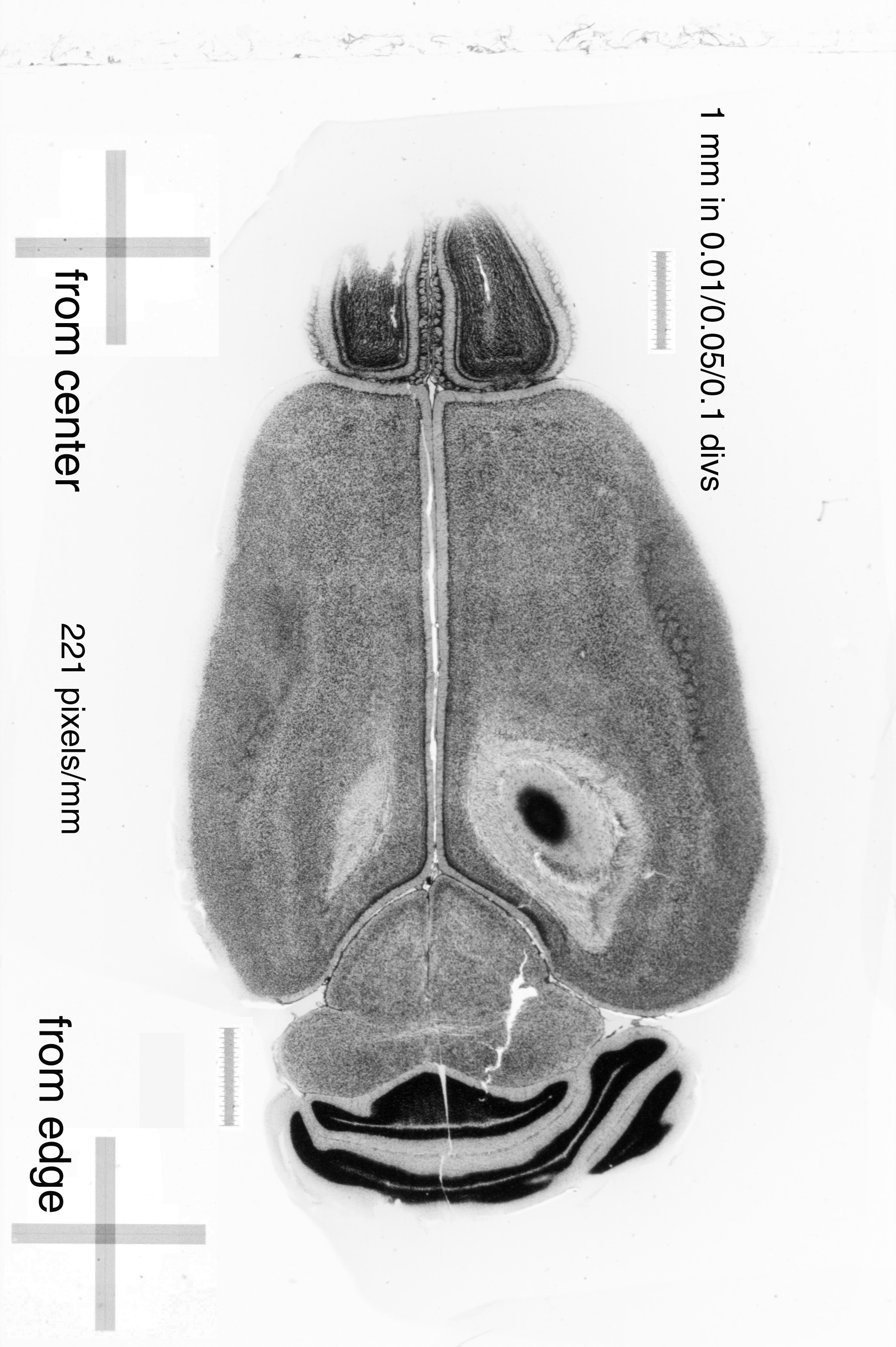
Calibration: For calibration of the images of individual sections in the MBL, please open Case 101, Slide A, Section 3 (JPEG, 0.8 MB, 2000 x 3000 pixels). Magnification is 221 pixels per mm; approximately 4.5 microns/pixel.

Shrinkage: We have computed shrinkage for a subset of approximately 120 brains in the MBL. Shrinkage during celloidin processing occurs during embedding and is relatively uniform in all directions. We find that the volumetric shrinkage averages 62.8% with a standard deviation of 3.6%. The residual volume of a brain is therefore typically 37% of its in vivo volume. The range of volumetric shrinkage across cases is from 57% to 71%. This marked variation probably reflects differences in the quality of fixation and the embedding processes. A volumetric shrinkage of 62.8% is equivalent to a uniform linear shrinkage of 28.1% (71.9% residual length) and an areal shrinkage of 48.3% (51.7% residual area).

Computing shrinkage of any case in the MBL is straightforward and simply involves comparing the brain weight (given for every case) with the estimated volume. The method of computing the volume of the brain after processing and cutting is detailed in point 8 of the tutorial on constructing your own mouse brain atlas.